New Mexico Tech
Earth and Environmental Science

ERTH 455 / GEOP 555 - Geodetic Methods

Lab 5: gd2p.pl: static position estimation

Note that you DO have to work on redoubt today!

Introduction

Last week I had you go through the motions of adding a new station to GIPSY's sta_info database and get used to processing with gd2p.pl. The processing, however, was quite arbitrary. I got you to a point where you know how to look at the postfit residuals. This week we will look a bit more into the various knobs you can use to improve the processing. You will look at residuals a lot (last week you figured out how to plot them), which show you how much the solution improves.

At this point I assume that you have successfully completed lab 4. You may need to go back to its description to lookup some of the details; opening it in a second browser tab is likely a good idea.

To keep myself out of trouble I should note that this lab follows a JPL workshop, but we're using our own data.

Setup

Below I show the sequence of commands that should get us all to the same starting point. Note that anything between redoubt and > is part of the prompt and not to be typed. The commands you will use start at the first space and range until the '#', which I use to comment what that line does.

	redoubt:~> cd $GEOP555                               #go to working directory
	redoubt:/data/GEOP555/gps>                           #'gps' part should be your user name! I am working as user 'gps'
	redoubt:/data/GEOP555/gps> mkdir lab05               #create folder to work in this week
	redoubt:/data/GEOP555/gps> cd lab05                  #go there
	redoubt:/data/GEOP555/gps/lab05>setenv WORKDIR `pwd` #creates the variable WORKDIR to refer to this place
	redoubt:/data/GEOP555/gps/lab05>echo $WORKDIR        #print the contents of this variable
	/data/GEOP/[USERNAME]/lab05/                         #this should be your output (USERNAME IS YOUR USERNAME) I will use this variable below!	
	

Whenever you log out and log back in, make sure to have $WORKDIR set to the value above. Obviously you don't have to create the lab05 directory every single time, as it will remain there.

If your $WORKDIR contains gps, you're doing it wrong!

Processing: Add Zenith Troposphere

Make a new directory for this run:

	$> mkdir $WORKDIR/run2
	$> cd $WORKDIR/run2
	

From last week's lab, copy the run_again script into $WORKDIR/run2. I assume that you worked in $GEOP555/lab04/run1:

    $> cp $GEOP555/lab04/run1/run_again ./r2
    $> cat r2											#should give you the output below (the 'gps' subdir should be your name)
    #!/bin/csh -f  

    #The following environment variables were active:
    #setenv GOA /usr/local/GIPSY/goa-6.3

    #You may need the following source command to set your PATH if you have changed it
    #source  /usr/local/GIPSY/goa-6.3/rc_gipsy.csh
    ( gd2p.pl \
          -i /data/GEOP555/gps/lab04/abbz2000.15o \
          -n ABBZ \
          -d 2015-07-19 \
          -r 300 \
          -type s \
          -w_elmin 15 \
          -e "-a 20 -PC -LC -F" \
          -pb_min_slip 1.0e-3 \
          -pb_min_elev 30 \
          -amb_res 2 \
          -dwght 1.0e-5 1.0e-3 \
          -post_wind 5.0e-3 5.0e-5 \
          -trop_z_rw -1.0 \
          -tides \
          -orb_clk "flinnR /data/GEOP555/gps/lab04/orbit" \
          -sta_info /data/GEOP555/gps/sta_info \
     > gd2p.log ) |&  sed '/^Skipping namelist/d' > gd2p.err
	

No surprises here! Exactly what you've done last week. Note that the stdout and stderr log files now are gd2p.log and gd2p.err, while they used to be run1.log and run1.err. That's alright. No need to change things. As we will be keeping our results in separate directories, there is no danger of overwriting results / logs.

Let's get to the wet troposphere. The current -1.0 is a negative value for parameter -trop_z_rw. If you read the documentation, you know that a negative value for this parameter means that it won't be estimated. That's purely instructional. Change this value to 5.0e-8 [km/sqrt(sec)] - this is a random walk value that is recommended from (JPL's) experience.

Save and execute the script:

    $> ./r2
	

If you list your directory contents, you the file EDIT_POINT_FAILURE didn't show up. gd2p.err should contain only warnings, no serious errors - the edit cycle converged! Yay! If you now compare the postfit residuals (LC) you will find them to be much smaller and the outliers are gone:

    redoubt:/data/GEOP555/gps/lab05/run2> cat ../../lab04/run1/Postfit.sum             #OLD RUN1
       start time         stop time      type  user      postfit sigma npts outliers
 
    15JUL18 23:59:43   15JUL19 23:54:43   LC   ABBZ      1.9478E-05    2073    434
    15JUL18 23:59:43   15JUL19 23:54:43   PC   ABBZ      4.4347E-04    2507      0
	
    redoubt:/data/GEOP555/gps/lab05/run2> cat Postfit.sum                              #RUN 2
       start time         stop time      type  user      postfit sigma npts outliers
 
    15JUL18 23:59:43   15JUL19 23:54:43   LC   ABBZ      1.1021E-05    2507      0
    15JUL18 23:59:43   15JUL19 23:54:43   PC   ABBZ      4.4397E-04    2507      0
	

Let's look at the residuals. I provide a script that creates the 2 file for lc and pc residuals that can be used for the plotting preparation: geop555_make_residuals.sh. This wraps the residual generation, data extraction, and file renaming that you've done by hand last week:

    redoubt:/data/GEOP555/gps/lab05/run2> geop555_make_residuals.sh 
    created:  run2_lc_res.txt run2_pc_res.txt
	

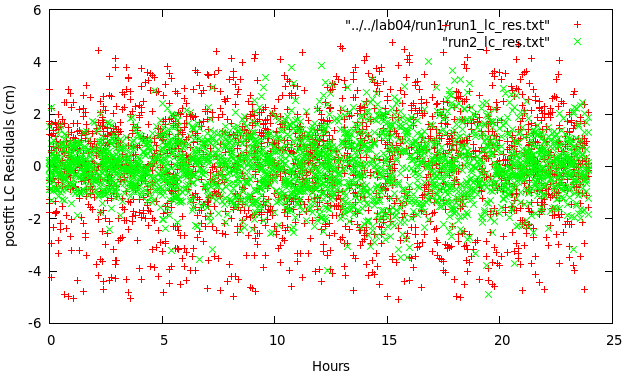
Now you can make the plots that compare previous and current residuals (we'll do that a lot):

    $> gnup -p ../../lab04/run1/run1_lc_res.txt run2_lc_res.txt -xl 'Hours' -yl 'postfit LC residuals (cm)'
	

You should get something like this:



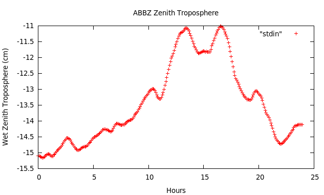
Clearly, the phase residuals are overall smaller, so we must have some wet troposphere, which our parameter represents better than no wet troposphere at all. Plot it with the script plot_wetz.sh that I provide (you need to provide the site ID as argument):

    $> plot_wetz.sh ABBZ
	

You should get something like this:



Definitely the code estimates some variation, with the most significant values at the beginning and end of the day (negative scale!).

The file tdp_* files contain information about the estimated parameters. The file tdp_final contains the final estimates:

• receiver clock is in field STA BIAS (km)
• phase biases per satellite PB GPSXX (km)
• station position STA X, STA Y, STA Z (km)
• dummy parameter used by filter DUM
• Now zenith troposphere estimates WETZTROP

    $> awk '{print $5,$6}' tdp_final | sort -u
	

If you were to look into the tdp file, you'll find a lot more. The meaning of the fields is documented here:

    $>  less $GOA/file_formats/tdp 
	

To get the position estimate you can use, as last week:

    $> grep "STA [XYZ]" tdp_final
	

Use xyz2wgs.py to convert the values into WGS84 positions. Note that you need to convert from kilometers to meters! How does this compare to the monument location that UNAVCO provides in the rinex file (lat =-77.4569; lon=166.9089; height=1734.2656)?

Adding Ocean and Earth Tides, Ionosphere

Make a new directory for this run and copy the r2 runscript:

    $> mkdir $WORKDIR/run3
    $> cd $WORKDIR/run3
    $> cp $WORKDIR/run2/r2 ./r3
	

Now for the parameters. Change the tides line to:

    -tides WahrK1 FreqDepLove OctTid PolTid \
	

WahrK1, FreqDepLove, OctTid invoke complete solid Earth tide models from IERS standards, PolTid invokes solid Earth pole tide from IERS standards.

Run it:

    $> ./r3
    

Produce a plot of the LC residuals of run3 compared to run1. Quite impressive, huh?

While we're at it, add an ocean load tide model (into r3, no need for a new directory if you've created the plot above!). Add the following lines into r3

    -add_ocnld \
    -OcnldCpn \
    -add_ocnldpoltid\
	

• add_ocnld adds 11 tidal frequencies: M2, S2, K2, N2, K1, O1, P1, Q1, Mf, Mm, Ssa.
• Default uses $GOA_VAR/sta_info/ocnld_coeff_cm_got48ac_wtpxo8ofunc
• can compute and add your own: -add_ocnld " -c your_coefficient_file"
• must be with respect to center of mass of earth system (solid earth and oceans)!
• OcnldCpn infers other tidal frequencies from 11 given ones
• add_ocnldpoltid adds Ocean load pole tide model - small improvement (12 and 14 month period)

Produce a plot of the LC residuals of run3 compared to run2.

Seems like it ran? Seems like you produced a new plot? Check gd2p.err! What's the error you are getting?

I have an oceanload model for the site ABBZ at $GIPSY/ocnload/tpxo72atlas_CM/gipsy/ABBZ.ocnld - add this to r3 as described above and rerun! (Note that the space is actually important!)

NOW: Produce a plot of the LC residuals of run3 compared to run2. A lot of the residuals in second half of day was due to tides!

Now we can add troposphere gradients (wetzgrad with recommended values), change the troposphere mapping function to something more modern (GPT2), and second order Ionosphere correction, as well as elevation dependent weighting using the sqrt(sin) of the elevation angle weight function.

      -wetzgrad 5.0e-9\
      -trop_map GPT2\
      -ion_2nd\
      -shell_height 600\
      -tec_mdl ionex\
      -ionex_file $GOA_VAR/etc/ionex/2015/201/jplg2010.15i.Z \
      -eldepwght SQRTSIN\
	

Produce another plot of the LC residuals of run3 compared to run2.

We're getting close (quite literally). However, we still have some work to do with respect to the antenna.

Antenna Phase Center Model

Make a new directory for this run and copy the r3 runscript:

    $> mkdir $WORKDIR/run4
    $> cd $WORKDIR/run4
    $> cp $WORKDIR/run3/r3 ./r4
    

Now, let's correct for the antenna phase center:

    $> grep ANT ../../lab04/abbz*o      #gives you the antenna information 
    

This gives you all the necessary information to create the antenna-phase-center correction file. Here is the example for ABBZ:

    $> antex2xyz.py -antexfile $GIPSY/pcenter/latest.atx -xyzfile ABBZ.xyz -radcode NONE -anttype TRM41249.00 -fel 0 -daz 5 -del 5 -extrap -recname ABBZ
    

This creates a file ABBZ.xyz in your local directory, which contains all the necessary information for antenna TRM41249.00 (a Zephyr Geodetic Antenna (check the P/N number on the picture!)). All that information comes from $GIPSY/pcenter/latest.atx the latest file containing this information, with maybe some extrapolation. Add this new file to your run script:

      -arp \
      -AntCal ABBZ.xyz\
    

Produce a plot of the LC residuals of run4 compared to run3. Not that much better? But check the WGS coordinates (with the table below)

What are the differences between nominal position and final solution for each run: run1 (last week), run2, run3 (final version), and run4 (subtract respective columns in tdp_final for the respective run); include the improvements in lat/lon/height estimates, too (convert XYZ2WGS and then difference) Give a table:

                 | run 1 - run 2 |  run2 - run3 | run3 - run4
    -------------+==============================================
    delta X      |
    delta Y      |
    delta Z      |
    delta lat    |
    delta lon    |
    delta height |
	
    

Deliverables: (submit via canvas, IN A ZIP FILE!)

• ABBZ position after troposphere correction
• Plot of the LC residuals with Earth tides removed (run3 vs run1)
• Plot of the LC residuals with Earth tides, ocean tides removed (run3 vs run2) - the fixed version!
• Table of position changes
• Final script r4